Quantum Reservoir Computing

Reservoir Computing (RC) in general leverages a fixed, randomly connected network structure called the ‘reservoir.’ This is in strong contrast to conventional deep learning architectures, which performe the optimization of weight across all layers. In RC, the reservoir enables dynamic, nonlinear transformations of input data into a high-dimensional feature space, followed by linear regression to produce the output. Quantum Reservoir Computing (QRC) tries to take advantage of the exponential scaling dimension of the Hilbert space in the quantum computing context to potentially provide an advantage over the classical RC. In QRC there is a register of accessable qubits \(\rho_0\), which are subject to encoding the classical information and measurements, and hidden qubits \(\rho_{\mathrm{hid}}\), which are related to the reservoir and artifically raise the dimension, the reservoir dynamic acts on, by the size of the hidden register. The hidden qubits can either be provided by an additional register or interaction with the enviroment.

First the classical input data \(x=\lbrace x^{(i)}\rbrace_{i=1}^D\), where \(D\) denotes the samplesize, gets related to a unitary evolution \(U(x)\), called encoding circuit, that evolves the initial state of the accessable qubits \(\rho_0\) to

\[\rho(x)=U(x)\rho_0U(x)^{\dagger}.\]

Afterwards the reservoir dynamic \(U_R\) gets applied to the composite of the accessable and hidden qubits, i.e

\[\tilde{\rho}(x)=U_R(\rho(x)\otimes \rho_{\mathrm{hid}})U_R^{\dagger}=U_R(U(x)\rho_0U(x)^{\dagger}\otimes \rho_{\mathrm{hid}})U_R^{\dagger}.\]

Now using a set of (usually randomized) observables \(\lbrace O_1, \ldots, O_M \rbrace\) the respective expecation- values

\[\langle O_j \rangle_x = \mathrm{Tr}(O_j \tilde{\rho}(x))\]

are deteremined by measurements for all \(j = 1 ,\ldots,M\). The resulting vector

\[\begin{split}\symbf{v}(x):= \begin{bmatrix}\langle O_1 \rangle_x\\\vdots\\\langle O_M \rangle_x\end{bmatrix}\end{split}\]

can be used to perform classical machine learning algorithms like linear regression. So the key advantage over QNN is that one does not optimize over the weights of a complex parametrized quantum circuit, but keeps the complex part fix and later optimizes the readout vectors via cheaper algorithms.

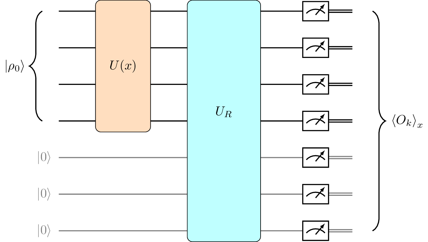
Figure 1 An example of a quantum reservoir computing circuit (see Ref. [1]). In the graphic we set the hidden qubits \(\rho_{\mathrm{hid}}\) as \(\ket{000}\). The encoding circuit (orange) and the quantum reservoir (blue) evolve the initial accessable qubit register \(\ket{\rho_0}\) and the composite of accessable and hidden qubits respectively. After the measurement with respect to the observable \(O_k\) we can repeat with similar circuits for all the other observables and use the expectation values to do classical machine learning.

Note that in sQUlearn, there is no hidden qubit register available in the pre-configured encoding circuits. This can be constructed manually if needed, or if run on a quantum computer, it may be due to the (non-controllable) interaction with the surrounding bath.

With the outputs of our QRC circuit we construct the so called readout vector

\[\symbf{v}^*(x)= \symbf{w}^\top \symbf{v}(x) = \sum\limits^M_{j=1} \symrm{w}_j \cdot \langle O_j \rangle_x,\]

where \(\symbf{w}^\top = (\symrm{w}_1, \ldots, \symrm{w}_M)\), and the task of classical maschine learning is to determine the best collection of weights \(\symrm{w}_j\). This can be done, for example, using a pseudo inverse method.

High-level methods for QRC

As already mentioned the expectation values \(\langle O_j \rangle_x\) will be used to carry out a classical maschine learning model. Usually one sticks to linear regression, since the complexity is transmitted to the reservoir. Nonetheless sQUlearn provides some additional options to choose from.

With sQUlearn it is possible to use QRC to do regression and classification tasks:

QRCClassifier	Quantum Reservoir Computing for classification.
QRCRegressor	Quantum Reservoir Computing for regression.

By passing either of both classes a fitting keyword argument mlp (multi-layer perceptron model), linear (linear model or single layer perceptron for classification) or kernel (support vector maschine) one can set the desired maschine learning model. We will now go step by step through the implementation of an example QRC for both methods with sQUlearn.

Classification

Setup

First an foremost the encoding of the classical data onto the accessable qubits and the quantum reservoir preparation is done in sQUlearn by the EncodingCircuit class. For details we refer to the documentations and examples in the user guidelines.

from squlearn.encoding_circuit import ChebyshevPQC

pqc = ChebyshevPQC(num_qubits=8, num_features=2, num_layers=2)
pqc.draw("mpl")

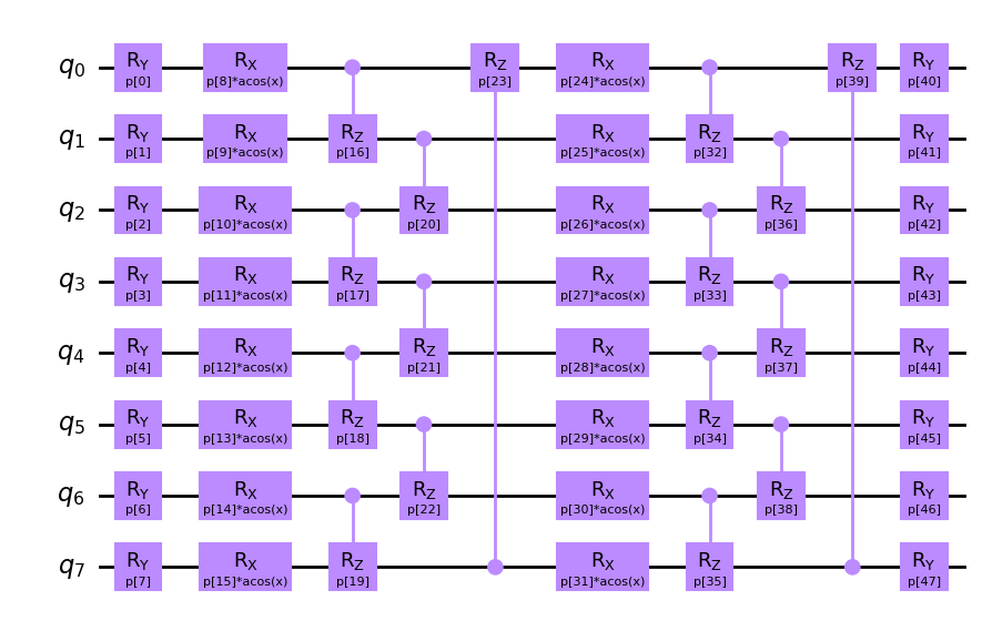
Here we have chosen the ChebyshevPQC as our encoding circuit, but sQUlearn provides a list of several alternative choices in Quantum Encoding Circuits. The parameters are all randomly chosen. Next we also initialize our executor and QRCClassifier:

from squlearn import Executor
from squlearn.qrc.qrc_classifier import QRCClassifier

exec = Executor()
qrc = QRCClassifier(pqc, executor=exec, ml_model="linear", num_operators=200)

The QRCClassifier takes our prepared EncodingCircuit and a machine learning method of our choice with linear regression as the default setting. In the last argument we can set the number of observables \(M\), which will be randomly chosen in order to measure the circuit and create the output vector \(\vec{v}\) of size \(M\). For closer instructions on the Executor class we refer to The Executor Class in the user guideline.

Training

Now we train our QRC model using the fit method after we specify a certain dataset we like to train on:

from sklearn.datasets import make_moons
from sklearn.model_selection import train_test_split
from sklearn.preprocessing import MinMaxScaler

X, y = make_moons(n_samples=1000, noise=0.2, random_state=42)

X_train, X_test, y_train, y_test = train_test_split(X, y, test_size=0.2, random_state=42)

scaler = MinMaxScaler(feature_range=(-0.9, 0.9))
X_train = scaler.fit_transform(X_train)
X_test = scaler.transform(X_test)

qrc.fit(X_train, y_train)

Result

In the end we can plot our results and see how it worked:

import numpy as np
import matplotlib.pyplot as plt

xx, yy = np.meshgrid(np.linspace(-1, 1, 50), np.linspace(-1, 1, 50))
Z = qrc.predict(np.c_[xx.ravel(), yy.ravel()])
Z = Z.reshape(xx.shape)

plt.contourf(xx, yy, Z, alpha=0.8)
plt.scatter(
    X_train[:, 0], X_train[:, 1], c=y_train, edgecolor="k", marker="X", label="Training Data"
)
plt.scatter(X_test[:, 0], X_test[:, 1], c=y_test, edgecolor="k", marker="o", label="Test Data")
plt.xlabel("Feature 1")
plt.ylabel("Feature 2")
plt.title("QRC Classification Inference")
plt.legend()
plt.show()

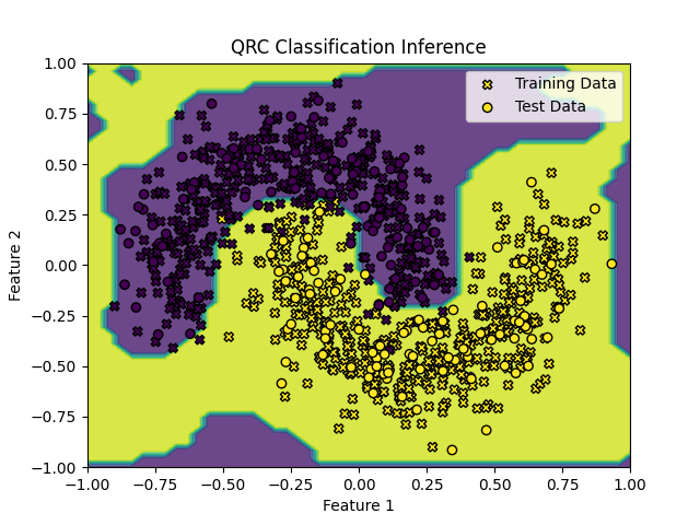
Figure 2 One can see that on this particular case the classification was very successful.

Regression

Setup

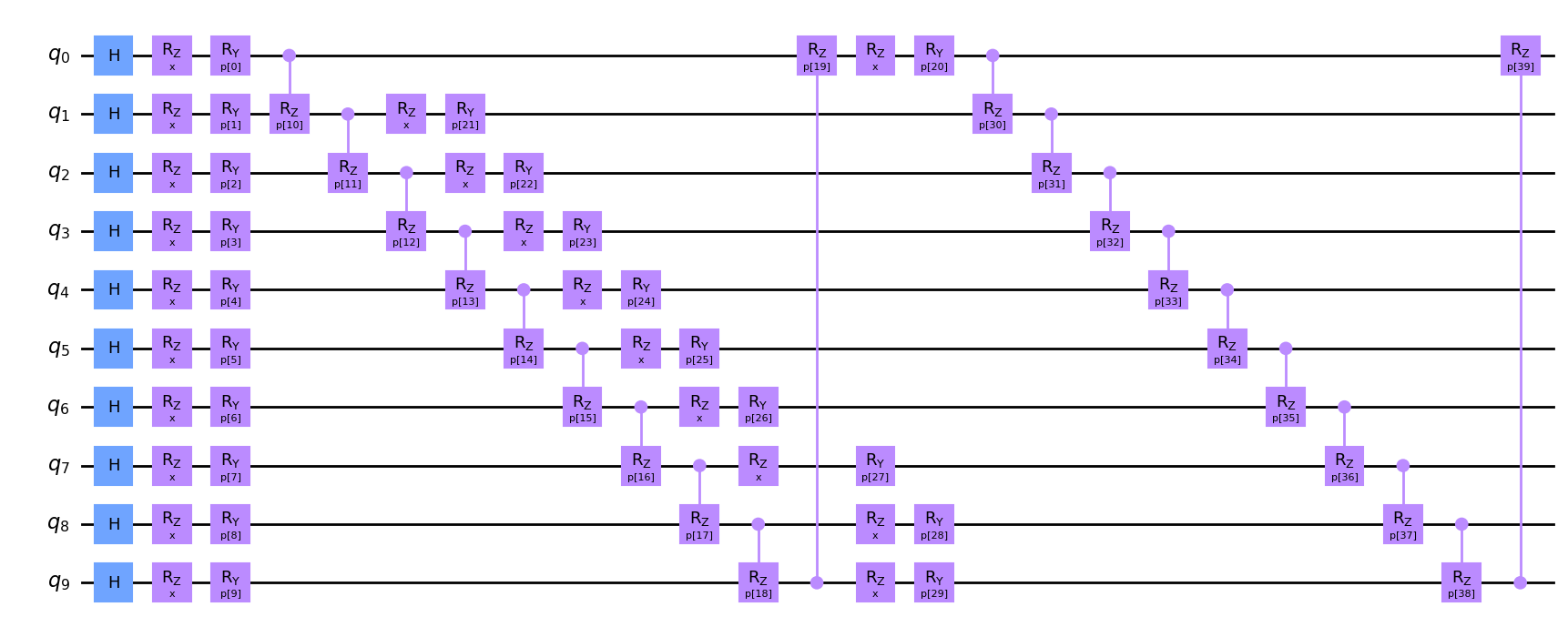
Just like in the classifier example we start by encoding the classical data and reservoir with the _encoding_circuit class. This time, we choose the HubregtsenEncodingCircuit as our encoding circuit, again with randomly picked parameters.

from squlearn.encoding_circuit import HubregtsenEncodingCircuit

pqc = HubregtsenEncodingCircuit(num_qubits=10, num_features=1, num_layers=2)
pqc.draw("mpl")

The QRCRegressor similar to the classifier example, takes our prepared EncodingCircuit and a machine learning method of our choice with linear regression as the default setting. In the last argument we again can determine the number of observables \(M\) to measure the circuit and create the output vector \(\vec{v}\) of size \(M\).

from squlearn import Executor
from squlearn.qrc import QRCRegressor

exec = Executor()
qrc = QRCRegressor(pqc, executor=exec, ml_model="linear", num_operators=200)

Training

import numpy as np

X_train = np.arange(0.0, 1.0, 0.1)
y_train = np.exp(np.sin(10 * X_train))
X_train = X_train.reshape(-1, 1)


X_test = np.arange(0.01, 1.0, 0.01)
y_test = np.exp(np.sin(10 * X_test))
X_test = X_test.reshape(-1, 1)

qrc.fit(X_train, y_train)

Now we evaluate the model by calculating the inference of the model and the training data set

y_pred = qrc.predict(X_test)

Result

import matplotlib.pyplot as plt
from sklearn.metrics import mean_squared_error, r2_score

print("Mean Squared Error:", mean_squared_error(y_test, y_pred))
print("R^2 Score:", r2_score(y_test, y_pred))

plt.plot(X_test, y_test, "-", color="blue", label="True Values")
plt.plot(X_test, y_pred, "-", color="red", label="Predictions")
plt.plot(X_train, y_train, "x", color="green", label="Training Set")
plt.xlabel("x")
plt.ylabel("f(x)")
plt.title("QRC Regression Inference")
plt.legend()
plt.show()

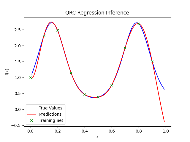
Figure 3 The regression of our discrete data set fits the function locally with high precision.

References

[1] Xiong, Weijie, et al. “On fundamental aspects of quantum extreme learning machines” arXiv:2312.15124 (2023).

[2] Suzuki, Y., Gao, Q., Pradel, K.C. et al. “Natural quantum reservoir computing for temporal information processing” Sci Rep 12, 1353 (2022).