Quantum Kernel Methods
Quantum Kernel Methods are among the most promising approaches to (supervised) Quantum Machine Learning (QML). This is due to the fact that it has been shown [1] that they can be formally embedded into the rich mathematical framework of classical kernel theory. The key idea in kernel theory is to solve the general task of machine learning, i.e. finding and studying patterns in data, in a high dimensional feature space - the reproducing kernel Hilbert space (RKHS) - where the original learning problem attains a trivial form. The mapping from the original space to the RKHS (which in general can be infinite-dimensional) is done by so called encoding circuits. The RKHS is endowed with an inner product which provides access to the high dimensional space without the need to ever explicitly calculate the high- (infinite-) dimensional feature vectors. This is known as the kernel trick: the encoding circuit and the inner product define a kernel function and vice versa, via
\(K(x,y) = \Braket{\phi(x), \phi(y)}\)
Due to the inner product, the kernel function formally computes the distance between data points \(x\) and \(y\) and thus effectively reduces to the illustrative interpretation of a similarity measure between data points.
The key point of Quantum Kernel methods is that they can be fundamentally formulated as a classical kernel method whose kernel is computed by a quantum computer. By using a quantum computer for the calculation of the kernel one naturally exploits the inherent quantum mechanical phenomena of superposition and entanglement - a fact which holds out the prospect of designing machine learning models that are able to deal with complex problems that are out of reach for conventional machine learning methods.
Quantum Kernel methods work analogously to their classical counterparts, with data embedded into the exponentially increasing quantum Hilbert space via a quantum encoding circuit
\(\ket{\psi(x,\boldsymbol{\theta})} = U_{\boldsymbol{\theta}}(x)\ket{0}\)
with \(U_{\boldsymbol{\theta}}(x)\) a parametrized quantum circuit for data encoding applied to the initial qubit state \(\ket{0}\) (as discussed below, trainable parameters can be introduced to optimally align a resulting quantum kernel to a given data set). This fundamental ansatz marks the bridge between QML and kernel methods. But for this to hold, we need to define the data encoding density matrices
\(\rho(x,\boldsymbol{\theta})=\ket{\psi(x,\boldsymbol{\theta})}\bra{\psi(x,\boldsymbol{\theta})}\)
as the feature “vectors”. Therefore, we can consider the space of complex density matrices enriched with the Hilbert-Schmidt inner product as the feature space of a quantum model and state [1]. In the quantum computational practice, the Hilbert-Schmidt inner products are revealed by measurements. Consequently, in quantum computing, access to the Hilbert space of quantum states is given by measurements.
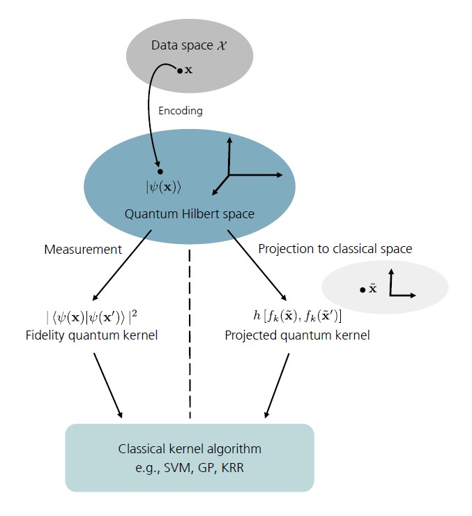
Figure 1 Schematic illustration of the function principle of quantum kernel methods, which can be formally embedded in the rich mathematical framework of conventional kernel theory. Data points \(\symbf{x}\) are mapped to the quantum Hilbert space by encoding them into a quantum state \(\ket{\symbf{\psi}(\symbf{x})}\). Access to the quantum Hilbert space is granted by measurements. \(\symbf{Left:}\) In quantum mechanics measurements are expressed through Hilbert-Schmidt inner products. Quantum kernels, which are defined using this fidelity-type metric are thus referred to as fidelity quantum kernels (FQKs). More on FQKs in sQUlearn will be discussed below. \(\symbf{Right:}\) When projecting the quantum states to an approximate classical representation using, e.g., reduced physical observables this gives rise to a family of projected quantum kernels (PQKs). These will be also subject to discussion in the sQUlearn context below.
High-Level methods that employ quantum kernels
In general, kernel methods refer to a collection of pattern analysis algorithms that use kernel functions to operate in a high-dimensional feature space. Probably, the most famous representative of these kernel-based algorithms is Support Vector Machines (SVMs). Kernel methods are most commonly used in supervised learning frameworks for either classification or regression tasks.
In the NISQ era (no access to fast linear algebra algorithms such as HHL), the basic notion of quantum kernel methods is to merely compute the kernel matrix with a quantum computer and subsequently pass it to an conventional kernel algorithms. For this task, sQUlearn provides a convenient workflow by either wrapping the corresponding scikit-learn estimators or by independently implementing them analogously, adapted to the needs of quantum kernel methods. sQUlearn offers SVMs for both classification (QSVC) and regression (QSVR) tasks, Gaussian Processes (GPs) for both classification (QGPC) and regression (QGPR) tasks as well as a quantum kernel ridge regression routine (QKRR).
Classification
In terms of classification algorithms, sQUlearn provides:
Quantum Support Vector Classification |
|
Quantum Gaussian process classification (QGPC), that extends the scikit-learn sklearn.gaussian_process.GaussianProcessClassifier. |
We refer to the documentations and examples of the respective methods for in-depth information and user guidelines.
Regression
In terms of regression algorithms, sQUlearn provides:
Quantum Support Vector Regression |
|
Quantum Kernel Ridge Regression. |
|
Quantum Gaussian Process Regression (QGPR). |
We refer to the documentations and examples of the respective methods for in-depth information and user guidelines.
Methods to evaluate quantum kernels
sQUlearn provides two methods to evaluate quantum kernels: Fidelity Quantum kernels (FQKs) and Projected Quantum kernels (PQKs), which also represent the standard approaches to quantum kernel methods in the literature.
Central to both approaches is the embedding of data into the quantum Hilbert space by using
quantum encoding circuits, which are nothing but encoding quantum circuits. These can optionally be
parametrized (as already implicitly introduced above) for optimally adjusting the resulting
quantum kernel to a given data set. If a encoding circuit with trainable parameters is used, sQUlearn
initializes them to some predefined and reasonable values, which can be controlled, within FQK
and PQK definitions via the argument parameter_seed (defaults to zero).
Beyond that, for both FQKs and PQKs, sQUlearn provides the option for regularizing the respective
kernel matrices using either thresholding or tikhonov approach as described in Ref. [2].
Regularization is by default switched of but can be set via the regularization
argument.
Fidelity Quantum Kernel (FQK) via FidelityKernel
The straightforward and natural way to the definition of a quantum kernel [1,3-5], is to use the native geometry of the quantum state space which is inherent in the Hilbert-Schmidt inner product, i.e.
\(k^Q(x,x^\prime)=\mathrm{tr}[\rho(x,\boldsymbol{\theta})\rho(x^\prime,\boldsymbol{\theta})]\)
which, for pure states, reduces to
\(k^Q(x,x^\prime)=\left|\Braket{\psi(x,\boldsymbol{\theta})|\psi(x^\prime, \boldsymbol{\theta})}\right|^2\),
i.e. a fidelity-type metric. From this, it immediately follows that evaluating the FQK scales quadratically in the data set size. Therefore, the applicability of FQKs is naturally restricted to small data set instances.
In sQUlearn a FQK (instance) can be defined as shown by the following example:
from squlearn.util import Executor
from squlearn.encoding_circuit import ChebyshevPQC
from squlearn.kernel import FidelityKernel
enc_circ = ChebyshevPQC(num_qubits=4, num_layers=2)
fqk_instance = FidelityKernel(
    encoding_circuit=enc_circ,
    executor=Executor()
)
When evaluating kernels on a real backend, sQUlearn provides an option for mitigating FQKs for
with respect to depolarizing noise using the approach discussed in Ref. [2]. The respective
mitigation technique uses the fact that ideally (train-train or test-test) kernel matrices
should consist exclusively of ones along the diagonal - a property which is by construction
fulfilled by PQKs. For FQKs one can attempt to restore this property using the
mit_depol_noise argument which can be either set to 'msplit' or 'mmean'
as defined in Ref. [2]. By default this option is set to None.
Projected Quantum Kernel (PQK) via ProjectedQuantumKernel
Several works show that with increasing problem size, the FQK approach suffers from exponential concentration leading to quantum models that suffer from untrainability. To circumvent this problem, Ref. [4] introduced a family of projected quantum kernels as a solution. These work by projecting the quantum states to an approximate classical representation by using, e.g., reduced physical observables.
The default PQK implementation of sQUlearn is one of the simplest forms of PQKs. They work by measuring the one-particle reduced density matrix (1-RDM) on all qubits for the encoded state and define the kernel as (RBF-inspired)
\(k^{PQ}(x,x^\prime)=\exp\left(-\gamma\sum_k\sum_{P\in\lbrace X,Y,Z\rbrace}\left[\mathrm{tr}(P\rho(x,\boldsymbol{\theta})_k) - \mathrm{tr}(P\rho(x^\prime,\boldsymbol{\theta})_k)\right]^2\right)\)
where \(\rho(x,\boldsymbol{\theta})_k=\mathrm{tr}_{j\neq k}\left[\rho(x,\boldsymbol{\theta})\right]\) refers to the 1-RDM, which is the partial trace of the quantum state \(\rho(x,\boldsymbol{\theta})=\ket{\psi(x,\boldsymbol{\theta})}\bra{\psi(x,\boldsymbol{\theta})}\) over all qubits except for the \(k\)-th qubit. After some lines of algebra, it can be seen that these \(\mathrm{tr}\) arguments are nothing but expectation values for measuring the Paulis \(X,Y,Z\) on each qubit in the state \(\ket{\psi(x,\boldsymbol{\theta})}\) and thus can be viewed as QNNs. The definition of PQKs is ambiguous. This concerns the outer form of the kernel, i.e. the function into which the QNN is put, the choice of observables used to evaluate the QNN as well as their respective locality, which eventually reflects in the order of RDMs used in the definition. Currently, sQUlearn implements different outer forms \(f(\cdot)\), which represent standard scikit-learn kernel functions (Gaussian, Matern, ExpSineSquared, RationalQuadratic, DotProduct, PariwiseKernel), i.e. generally speaking, sQUlearn provides PQKs of the form
\(k^{PQ}(x,x^\prime) = f\left[QNN(x), QNN(x^\prime)\right]\)
A respective PQK (instance) referring to the definition given above is defined as illustrated by the following example:
from squlearn.util import Executor
from squlearn.encoding_circuit import ChebyshevPQC
from squlearn.kernel import ProjectedQuantumKernel
enc_circ = ChebyshevPQC(num_qubits=4, num_layers=2)
pqk_instance = ProjectedQuantumKernel(
    encoding_circuit=enc_circ,
    executor=Executor(),
    measurement='XYZ',
    outer_kernel='gaussian'
)
Moreover, the QNNs can be evaluated with respect to different observables, where in
addition to the default setting - measurement='XYZ' - one can specify measurement='X',
measurement='Y' and measurement='Z' for one-qubit measurements with respect to only
one Pauli operator. Beyond that, one can also specify an observable or a list of observables, see the
respective examples in ProjectedQuantumKernel or the Observables for expectation values
user guide.
Training of quantum kernels
As mentioned above, the definition of quantum kernels (both FQK and PQK) relies quantum encoding circuits that are represented through parametrized quantum circuits (PQC). This results in quantum kernels that contain trainable parameters to optimally adjust to a given learning problem. The trainable parameters are obtained from classical optimization loops which attempt to minimize a given loss function.
sQUlearn implements the kernel target alignment procedure as well as the Negative-Log-Likelihood.
At the same time it provides several optimizers such as Adam and SLSQP;
This can be achieved by employing the KernelOptimizer class which automatically
enables the optimization of quantum kernels when used in the high-level methods.
The following examples assume that you have some data set available which you previously split into training and test data and shows how to optimize kernels.
Example - Kernel Target Alignment
from squlearn.util import Executor
from squlearn.encoding_circuit import ChebyshevPQC
from squlearn.optimizers import Adam
from squlearn.kernel import ProjectedQuantumKernel, KernelOptimizer, QKRR
from squlearn.kernel.loss import TargetAlignment

# set up the encoding circuit
encoding_circuit = ChebyshevPQC(num_qubits=4, num_layers=2)

# set up the quantum kernel
pqk_instance = ProjectedQuantumKernel(encoding_circuit, Executor())

# set up the optimizer
adam_opt = Adam(options={"maxiter":100, "lr": 0.1})

# define KTA loss function
kta_loss = TargetAlignment()

# set up the kernel optimizer
kernel_optimizer = KernelOptimizer(quantum_kernel=pqk_instance, loss=kta_loss, optimizer=adam_opt)

# initialize the QKRR model with the kernel optimizer
qkrr = QKRR(kernel_optimizer)

# Simple example
x_train = [[0.1], [0.2], [0.3], [0.4], [0.5]]
y_train = [0.1, 0.2, 0.3, 0.4, 0.5]
qkrr.fit(X=x_train, y=y_train)
References
[4] S. Jerbi et al., “Quantum machine learning beyond kernel methods”. arXiv:2110.13162v3 (2023)
[5] H. Y. Huang et al., “Power of data in quantum machine learning”. Nat. Commun. 12, 2631 (2021).