Quantum Neural Networks

Quantum Neural Networks (QNNs) extend the concept of artificial neural networks into the realm of quantum computing. Typically, they are constructed by encoding input data into a quantum state through a sequence of quantum gates. This quantum state is then manipulated using trainable parameters and utilized to evaluate an expectation value of an observable that acts as the output of the QNN. This output is then used to calculate a loss function, which is subsequently minimized by a classical optimizer. The resultant QNN can then be employed to predict outcomes for new input data.

In many cases, QNNs adhere to a layered design, akin to classical neural networks, as illustrated in figure 1. However, it is essential to note that they do not adhere to the concept of neurons as seen in classical neural networks. Therefore, the term “Quantum Neural Network” may be somewhat misleading, as QNNs do not conform to the traditional neural network paradigm. Nevertheless, their application domain closely resembles that of classical neural networks, which explains the established nomenclature.

Figure 1 Layered design of a QNN with alternating encoding (orange) and parameter (blue) layers. The QNN is trained in a hybrid quantum-classical scheme by optimizing the QNN’s parameters \({\theta}\) for a given cost function \(L\).

In principle, the design of QNN architectures offers a high degree of freedom. Nevertheless, most common designs follow a layered structure, where each layer comprises an encoding layer denoted as \(U_i({x})\) and a parameterized layer represented as \(U_i({\theta})\). The encoding layers map the input data, \({x}\), to a quantum state of the qubits, while the parameterized layers are tailored to modify the mapped state.

The selection of the encoding method depends on the specific problem and the characteristics of the input data, whereas parameterized layers are explicitly designed to alter the mapped state. Furthermore, entanglement among the qubits is introduced, enabling the QNN to process information in a more intricate and interconnected manner. Finally, we repeatedly measure the resulting state, denoted as \(\Psi({x}, {\theta})\), to evaluate the QNN’s output as the expectation value:

\[f({x}, {\theta}) = \langle\Psi({x}, {\theta}) \lvert\hat{C}({\theta}) \rvert\Psi({x}, {\theta}) \rangle\]

Here, \(\hat{C}({\theta})\) represents a operator, also called observable, for each output of the QNN. While the observable can be freely selected, it often involves operators based on a specific type of Pauli matrices, such as the Pauli Z matrix, to simplify the evaluation of the expectation.

It’s worth noting that both the embedding layers \(U_i({x})\) and the observable \(\hat{C}\) may also contain additional trainable parameters.

To train Quantum Neural Networks (QNNs), a hybrid quantum-classical approach is employed. The training process consists of two phases: quantum circuit evaluation and classical optimization (as illustrated in figure 1).

In the quantum circuit evaluation phase, the QNN and its gradient with respect to the parameters are assessed using a quantum computer or simulator. The gradient can be obtained using the parameter-shift rule. Subsequently, in the classical optimization phase, an appropriate classical optimization algorithm is employed to update the QNN’s parameters. This iterative process is repeated until the desired level of accuracy is attained.

Commonly used classical optimizers, such as SLSQP (for simulators) or stochastic gradient descent, like Adam, are applied in the classical optimization stage of QNN training. They adjust the QNN’s parameters to minimize a predefined cost function, denoted as \(L\):

\[\min_{\theta} L(f, {x}, {\theta})\]

The specific form of the cost function depends on the problem that the QNN is designed to solve. For instance, in a regression problem, the cost function is often defined as the mean squared error between the QNN’s output and the target value.

High-level methods for QNNs

In this section, we will illustrate the process of constructing a QNN using sQUlearn. A QNN is composed of two main components: an encoding circuit, which is essentially a parameterized quantum circuit, and a cost operator.

In sQUlearn, we have dedicated classes for these components: EncodingCircuit and CostOperator, both of which we will utilize in the upcoming example.

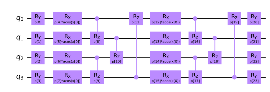
In the following cell, we will build an encoding circuit based on the Chebyshev input encoding method:

from squlearn.encoding_circuit import ChebyshevPQC

pqc = ChebyshevPQC(num_qubits = 4, num_features = 1, num_layers = 2)
pqc.draw("mpl")

There are several alternative encoding circuits at your disposal in sQUlearn, which you can explore in the user guide located at Quantum Encoding Circuits.

The second ingredient is to specify an observable for computing the QNN’s output. In this particular example, we employ a summation over a Pauli Z observable for each qubit, along with a constant offset:

from squlearn.observables import SummedPaulis

op = SummedPaulis(num_qubits=4)
print(op)

SparsePauliOp(['IIII', 'IIIZ', 'IIZI', 'IZII', 'ZIII'],
              coeffs=[ParameterExpression(1.0*p[0]), ParameterExpression(1.0*p[1]),
 ParameterExpression(1.0*p[2]), ParameterExpression(1.0*p[3]),
 ParameterExpression(1.0*p[4])])

Other expectation operators can be found in the user guide on Observables for expectation values.

Now we can construct a QNN from the encoding circuit and the cost operator. sQUlearn offers two easy-to-use implementation of QNNs, either for regression or classification:

QNNClassifier	Quantum Neural Network for Classification.
QNNRegressor	Quantum Neural Network for Regression.

We refer to the documentations and examples of the respective classes for in-depth information.

In the following example we will use a QNNRegressor, the encoding circuit, and the observable as defined above. Additionally, we utilize the mean squared error loss function and the Adam optimizer for optimization.

from squlearn.observables import SummedPaulis
from squlearn.encoding_circuit import ChebyshevPQC
from squlearn.qnn import QNNRegressor, SquaredLoss
from squlearn.optimizers import Adam
from squlearn import Executor

op = SummedPaulis(num_qubits = 4)
pqc = ChebyshevPQC(num_qubits = 4, num_features = 1, num_layers = 2)
qnn = QNNRegressor(pqc, op, Executor(), SquaredLoss(), Adam())

The QNN can be trained utilizing the fit method:

import numpy as np
# Data that is inputted to the QNN
x_train = np.arange(-0.5, 0.6, 0.1)
# Data that is fitted by the QNN
y_train = np.square(x_train)

qnn.fit(x_train, y_train)

The inference of the QNN is calculated using the predict method:

x_test = np.arange(-0.5, 0.5, 0.01)
y_pred = qnn.predict(x_test)

Optimization

sQUlearn offers a lot of possibilities to train a QNN’s parameters. In this section we will show, how to use SLSQP, as an example for a wrapped scipy optimizer, and Adam with mini-batch gradient descent to optimize the loss function.

SLSQP

sQUlearn offers wrapper functions, SLSQP and LBFGSB, for scipy’s SLSQP and L-BFGS-B implementations as well as the wrapper function SPSA for Qiskit’s SPSA implementation. We show how to import and use SLSQP in the following code block, other optimization methods can be used analogously.

from squlearn.optimizers import SLSQP

...
slsqp = SLSQP(options={"maxiter": 100})
...
reg = QNNRegressor(
    ...
    optimizer=slsqp,
    ...
)

With this configuration, QNNRegressor will use scipy’s minimize function with method="SLSQP". The wrapper Class SLSQP allows to specify hyper parameters in a dict that get passed on to the function.

Mini-Batch gradient descent with Adam

sQUlearn’s QNN classes, QNNRegressor and QNNClassifier, also offer the possibility to use mini-batch gradient descent with Adam to optimize the model. This allows for training on bigger data sets. Therefore we import and use the Adam optimizer as demonstrated in the following code block.

from squlearn.optimizers import Adam

...

adam = Adam(options=options_dict)

...

reg = QNNRegressor(
    ...
    optimizer=adam,
    ...
    batch_size=batch_size,
    epochs=epochs,
    shuffle=True,
    ...
)

Using SGD optimizers like the Adam optimizer allows us to specify further hyper parameters such as batch_size, epochs and shuffle. The parameters batch_size and epochs are positive numbers of type int and shuffle is a bool which specifies, whether data points are shuffled before each epoch.

Schedule of the learning rate of Adam

Sometimes it can be beneficial to adjust the learning rate of the optimizer during the training. This is possible by providing a List or a Callable to the learning rate option lr of the Adam optimizer. Then a learning rate is chosen from the list or calculated by the callable at the beginning of each iteration or epoch. A suitable function for generating a callable with an exponential decay of the learning rate is provided by get_lr_decay(). The following example will generate an Adam optimization with an exponential decay in the learning rate from 0.01 to 0.001 over 100 iterations.

from squlearn.optimizers import Adam
from squlearn.qnn import get_lr_decay
adam = Adam({'lr':get_lr_decay(0.01, 0.001, 100)})

Dynamically adjustments of the shots

It is possible to adjust the number of shots for the gradient evaluation. The number of shots are calculated from the relative standard deviation (RSTD) of the Loss function \(L\). Objective is that the RSTD should be smaller than a given threshold \(\beta\).

\[\text{RSTD}(L) = \frac{\sqrt{\frac{\sigma_L^2}{N_\text{shots}}}}{L} < \beta\]

The high-level implementations of QNNs, QNNRegressor and QNNClassifier, can be initialized with a shot controller that takes care to automatically adjust the number of shots. The following example will generate a QNNRegressor with a RSTD threshold of 0.1 and a minimum and maximum number of shots of 100 and 10000. It utilizes the ShotsFromRSTD shot controller.

from squlearn.qnn import QNNRegressor, ShotsFromRSTD
reg = QNNRegressor(
    ...
    shot_controller = ShotsFromRSTD(rstd_bound=0.1,min_shots=100,max_shots=10000),
    ...
)

Together with the variance reduction described in the next section, this allows to reduce the number of shots in the early stages of the optimization significantly and increase them in the later stages when a higher accuracy is required.

Variance reduction

When evaluating a pretrained QNN on Qiskit’s QasmSimulator or on real hardware, the model output will be subject to randomness due to the finite number of shots. The noise level of the model thus depends on its variance, which can be calculated as

\[\sigma_f^2 = \langle\Psi\lvert\hat{C}^2\rvert\Psi\rangle - \langle\Psi\lvert\hat{C}\rvert\Psi\rangle^2 \text{.}\]

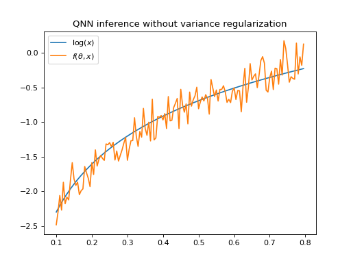
Figure 2 shows the output of a QNNRegressor fit to a logarithm with SquaredLoss evaluated on Qiskit’s QasmSimulator. The model has been trained with a noise-free simulator, but evaluating it on a noisy simulator yields a high variance in the model output.

(Source code, png, hires.png, pdf)

Figure 2 Logarithm and output of QNNRegressor \(f(\theta, x)\) evaluated on Qiskit’s QasmSimulator. The QNN output has a high variance.

We can mitigate this problem by adding the models variance to the loss function \(L_\text{fit}\) and thus regularizing for variance. We do this by setting the variance keyword in the initialization of the QNNRegressor (or QNNClassifier) with a hyper-parameter \(\alpha\).

reg = QNNRegressor(
    ...
    variance = alpha,
    ...
)

The new total loss function reads as

\[L_\text{total} = L_\text{fit} + \alpha \cdot \sum_k \lVert \sigma_f^2 ( x_i )\rVert \text{,}\]

where \(\sigma_f^2( x_i )\) is the variance of the QNN on the training data \(\{x_i\}\).

The regularization factor \(\alpha\) controls the influence of the variance regularization on the total loss. It can be either set to a constant float or a Callable that takes the keyword argument iteration to dynamically adjust the factor. Values between \(10^{-2}\) and \(10^{-4}\) have shown to yield satisfying results. [1]

Evaluation on Qiskit’s QasmSimulator now yields less variance in the model, as depicted in figure 3.

(Source code, png, hires.png, pdf)

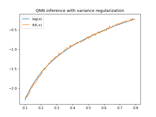
Figure 3 Logarithm and output of QNNRegressor \(f(\theta, x)\), trained with variance regularization, evaluated on Qiskit’s QasmSimulator. The QNN output has a low variance.

Variance reduction with dynamic adjustment of the regularization factor

Furthermore it is possible to adjust the variance regularization factor dynamically during the optimization. This allows for example to prioritize the minimization of the variance in the early stages of the optimization and then focus on the minimization of the loss function in the later stages (see Ref. [1]). This can be achieved by passing a List or a Callable to the keyword argument variance of the QNNRegressor (or QNNClassifier). The following example will generate a QNNRegressor with a variance regularization factor that is adjusted dynamically during the optimization by utilizing the function get_variance_fac(). The set-up features a final regularization factor of 0.005, a decay factor of 0.08 and a plateau at \(\alpha=1\) of 20 iterations at the beginning.

from squlearn.qnn import QNNRegressor,get_variance_fac
reg = QNNRegressor(
    ...
    variance = get_variance_fac(0.005,0.08,20),
    ...
)

References

[1] D. A. Kreplin and M. Roth “Reduction of finite sampling noise in quantum neural networks”. arXiv:2306.01639 (2023).