Hyperparameter Optimization and Pipelines
Summary
This tutorial demonstrates how to integrate quantum machine learning algorithms, specifically quantum kernel methods, from the squlearn library with traditional machine learning workflows in scikit-learn. We’ll go through data generation, preprocessing, model definition, and hyperparameter optimization using GridSearchCV. The objective is to highlight that squlearn algorithms can be seamlessly used alongside classical algorithms.
Importing Libraries
In this initial cell, we are importing all the libraries required for the tutorial. We are using squlearn for quantum kernel methods like Quantum Support Vector Regression (QSVR) and Quantum Gaussian Process Regression (QGPR). For tasks like data scaling and hyperparameter optimization, we rely on scikit-learn.
[1]:
import matplotlib.pylab as plt
import numpy as np
import pandas as pd
import seaborn as sns

from sklearn.model_selection import GridSearchCV
from sklearn.pipeline import Pipeline
from sklearn.preprocessing import StandardScaler

from squlearn import Executor
from squlearn.encoding_circuit import YZ_CX_EncodingCircuit
from squlearn.kernel.lowlevel_kernel import FidelityKernel, ProjectedQuantumKernel
from squlearn.kernel import QGPR, QSVR
Generating Data
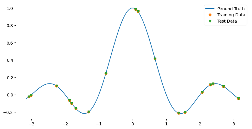
Here, synthetic data is generated. We sample a training data set where we perform a grid search on. We also create hold-out test data which will be used to score the best estimator of the grid search.
[2]:
def generate_y(x):
    u = x * np.pi
    return np.sin(u) / u


np.random.seed(42)

# define training and test data
x = np.linspace(-np.pi, np.pi, 100)
y = generate_y(x)
x_train = np.random.choice(x, 20)
y_train = generate_y(x_train)

x_test = np.random.choice(x, 20)
y_test = generate_y(x_test)

plt.figure(figsize=(10, 5))
plt.plot(x, y, label="Ground Truth")
plt.plot(x_train, y_train, "o", label="Training Data")
plt.plot(x_train, y_train, "v", label="Test Data")
plt.legend()
[2]:
<matplotlib.legend.Legend at 0x1b64e35ee30>
Setting up the kernels
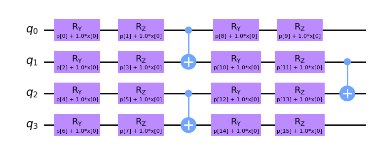
We want to compare two QML algorithms with the same encoding circuit and two variants of calculating the kernel: Fidelity kernels and projected quantum kernels. We set up the encoding circuit with initial parameters. These will be varied during the grid search. The kernel instances are initialized using Qiskit’s StatevectorSimulator.
[3]:
encoding_circuit = YZ_CX_EncodingCircuit(num_qubits=4, num_layers=2, closed=False)

executor = Executor()

fidelity_kernel = FidelityKernel(
    encoding_circuit=encoding_circuit, executor=executor, parameter_seed=0
)
projected_kernel = ProjectedQuantumKernel(
    encoding_circuit=encoding_circuit, executor=executor, parameter_seed=0
)

encoding_circuit.draw("mpl", num_features=1)
[3]:
Setting up the grid search
In this section, we define the quantum kernel methods we’ll be using for regression: Quantum Support Vector Regression (QSVR) and Quantum Gaussian Process Regression (QGPR). We initialize both with the two kernel-variants from above
We use GridSearchCV from sklearn to perform hyperparameter optimization. The hyperparameters include the number of qubits and layers for the quantum encoding circuits.
[4]:
num_qubit_list = [1, 2, 4]
num_layers_list = [1, 2, 3]

encoding_circuit_params = {
    "estimator__num_qubits": num_qubit_list,
    "estimator__num_layers": num_layers_list,
}

estimator_list = [
    QGPR(quantum_kernel=fidelity_kernel, full_regularization=False),
    QGPR(quantum_kernel=projected_kernel, full_regularization=False),
    QSVR(quantum_kernel=fidelity_kernel),
    QSVR(quantum_kernel=projected_kernel),
]

param_grid = []
for estimator in estimator_list:
    estimator_params = encoding_circuit_params.copy()
    estimator_params["estimator"] = [estimator]
    param_grid.append(estimator_params)
To scale the data, we use scikit-learns StandardScaler. This ensures that each feature has a mean of 0 and a standard deviation of 1, making it easier for the model to learn the optimal parameters. We create a pipeline with data scaling and the estimator to ensure that data scaling is part of the cross-validation process. We initialize the pipeline with an estimator. This will be overwritten in the grid search.
[5]:
pipeline = Pipeline(
    [("scaler", StandardScaler()), ("estimator", QGPR(quantum_kernel=fidelity_kernel))]
)
Running Grid Search
Now that everything is set up, we execute the grid search by fitting it to the training data. GridSearchCV will evaluate every combination of hyperparameters and choose the best set for each estimator (QSVR and QGPR in this case) based on the mean test score.
[6]:
grid_search = GridSearchCV(pipeline, param_grid, scoring="neg_mean_squared_error")
grid_search.fit(x_train.reshape(-1, 1), y_train)
[6]:
GridSearchCV(estimator=Pipeline(steps=[('scaler', StandardScaler()),
                                       ('estimator',
                                        QGPR(quantum_kernel=<squlearn.kernel.lowlevel_kernel.fidelity_kernel.FidelityKernel object at 0x000001B64E35C2E0>))]),
             param_grid=[{'estimator': [QGPR(full_regularization=False,
                                             quantum_kernel=<squlearn.kernel.lowlevel_kernel.fidelity_kernel.FidelityKernel object at 0x000001B64E...
                          'estimator__num_qubits': [1, 2, 4]},
                         {'estimator': [QSVR(C=1.0, cache_size=200, epsilon=0.1,
                                             max_iter=-1,
                                             quantum_kernel=<squlearn.kernel.lowlevel_kernel.projected_quantum_kernel.ProjectedQuantumKernel object at 0x000001B64E333E50>,
                                             shrinking=True, tol=0.001,
                                             verbose=False)],
                          'estimator__num_layers': [1, 2, 3],
                          'estimator__num_qubits': [1, 2, 4]}],
             scoring='neg_mean_squared_error')
In a Jupyter environment, please rerun this cell to show the HTML representation or trust the notebook. On GitHub, the HTML representation is unable to render, please try loading this page with nbviewer.org.
GridSearchCV(estimator=Pipeline(steps=[('scaler', StandardScaler()),
                                       ('estimator',
                                        QGPR(quantum_kernel=<squlearn.kernel.lowlevel_kernel.fidelity_kernel.FidelityKernel object at 0x000001B64E35C2E0>))]),
             param_grid=[{'estimator': [QGPR(full_regularization=False,
                                             quantum_kernel=<squlearn.kernel.lowlevel_kernel.fidelity_kernel.FidelityKernel object at 0x000001B64E...
                          'estimator__num_qubits': [1, 2, 4]},
                         {'estimator': [QSVR(C=1.0, cache_size=200, epsilon=0.1,
                                             max_iter=-1,
                                             quantum_kernel=<squlearn.kernel.lowlevel_kernel.projected_quantum_kernel.ProjectedQuantumKernel object at 0x000001B64E333E50>,
                                             shrinking=True, tol=0.001,
                                             verbose=False)],
                          'estimator__num_layers': [1, 2, 3],
                          'estimator__num_qubits': [1, 2, 4]}],
scoring='neg_mean_squared_error')Pipeline(steps=[('scaler', StandardScaler()),
('estimator',
QGPR(quantum_kernel=<squlearn.kernel.lowlevel_kernel.fidelity_kernel.FidelityKernel object at 0x000001B64E35C2E0>))])StandardScaler()
QGPR(quantum_kernel=<squlearn.kernel.lowlevel_kernel.fidelity_kernel.FidelityKernel object at 0x000001B64E35C2E0>)
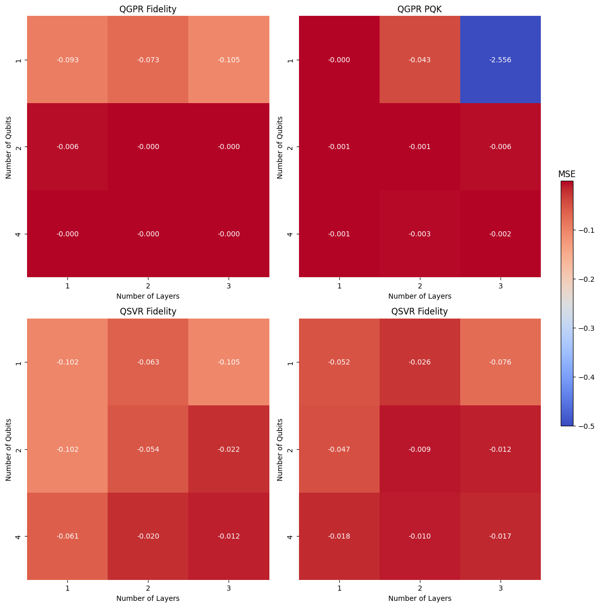
Results Analysis
To visualize the performance of different hyperparameter combinations, we plot heat maps for each estimator. Each cell in the heat map represents a combination of the number of qubits and layers used in the quantum encoding circuit, and the color represents the negative mean test score (MSE, larger is better). This allows for an intuitive understanding of how different hyperparameters impact performance.
[14]:
# Extract the results into a DataFrame
results_df = pd.DataFrame(grid_search.cv_results_)

# Number of unique combinations per estimator
num_combinations = len(num_qubit_list) * len(num_layers_list)

# Number of estimators
num_estimators = len(estimator_list)

# Initialize the grid for subplots
n_rows = int(np.ceil(np.sqrt(num_estimators)))
n_cols = int(np.ceil(num_estimators / n_rows))

fig, axs = plt.subplots(n_rows, n_cols, figsize=(12, 12), constrained_layout=True)

# Flatten the axis array for easier indexing
if n_rows > 1 or n_cols > 1:
    axs = axs.flatten()

# Set min and max for the colormap
vmin = -0.5
vmax = results_df["mean_test_score"].max()

estimator_names = ["QGPR Fidelity", "QGPR PQK", "QSVR Fidelity", "QSVR Fidelity"]
# Loop through the chunks to plot each heat map
for i in range(num_estimators):
    start_idx = i * num_combinations
    end_idx = (i + 1) * num_combinations
    chunk_df = results_df.iloc[start_idx:end_idx]

    # Pivot to get a matrix form suitable for heat maps
    heat_map_data = chunk_df.pivot_table(
        index="param_estimator__num_qubits",
        columns="param_estimator__num_layers",
        values="mean_test_score",
    )

    # Create the heat map (cbar=False will disable individual colorbars)
    sns.heatmap(
        heat_map_data,
        annot=True,
        fmt=".3f",
        cmap="coolwarm",
        ax=axs[i],
        vmin=vmin,
        vmax=vmax,
        cbar=False,
    )
    axs[i].set_title(f"{estimator_names[i]}")
    axs[i].set_xlabel("Number of Layers")
    axs[i].set_ylabel("Number of Qubits")

# Add a colorbar with label
cbar = fig.colorbar(
    axs[-1].collections[0],
    ax=axs,  # über alle Subplots verteilt
    location="right",  # automatisch rechts außen
    fraction=0.02,
    pad=0.02,
    label="MSE",
)

plt.show()
The best performing estimator is now evaluated on the test set and its predictions are shown alongside the generating data.
[8]:
# Get the best estimator
best_estimator = grid_search.best_estimator_

# Score the best estimator on the test set
test_score = best_estimator.score(x_test.reshape(-1, 1), y_test)
print(f"Test Score: {test_score}")

# Make predictions on the test set
y_pred = best_estimator.predict(x_test.reshape(-1, 1))

# Plot the predictions and ground truth
plt.figure(figsize=(10, 5))
plt.plot(x, y, label="Ground Truth")
plt.scatter(x_test, y_pred, c="red", label="Predictions")
plt.xlabel("X")
plt.ylabel("Y")
plt.title("Predictions vs Ground Truth")
plt.legend()
plt.show()
Test Score: 0.999999978217105
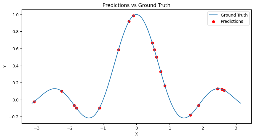
Note that in the above evaluation, the QSVR did not perform quite as good as the QGPR. The QSVR is, as its classical counterpart, sensitive to additional hyperparameters which have not been varied during the grid search. We now include the classical regularization parameter C and the slack variable epsilon as additional parameters in the search. This also demonstrates that parameters of the quantum kernel and parameters of the classical algorithm can be treated equally during the search.
[9]:
QSVR(quantum_kernel=fidelity_kernel)

estimator_params = encoding_circuit_params.copy()
estimator_params["estimator"] = [QSVR(quantum_kernel=fidelity_kernel)]
estimator_params["estimator__C"] = [1e0, 1e1, 1e2]
estimator_params["estimator__epsilon"] = [1e-4, 1e-3, 1e-2]
param_grid = estimator_params

grid_search = GridSearchCV(pipeline, param_grid, scoring="neg_mean_squared_error")
grid_search.fit(x_train.reshape(-1, 1), y_train)

print(f"Best Score: {grid_search.best_score_}")
print(f"Best Estimator: {grid_search.best_estimator_}")
Best Score: -3.020475311434476e-05
Best Estimator: Pipeline(steps=[('scaler', StandardScaler()),
                ('estimator',
                 QSVR(C=100.0, cache_size=200, epsilon=0.0001, max_iter=-1,
                      quantum_kernel=<squlearn.kernel.lowlevel_kernel.fidelity_kernel.FidelityKernel object at 0x000001B65219AC20>,
                      shrinking=True, tol=0.001, verbose=False))])
With these more adequate classical hyperparameters, the QSVR performs similarly to the QGPR.